Contract Report for HIBECO
EU Project
Download the report (MS-WORD
format, 2.9M) and resultant images (Idrisi32
format, 5.6M)
The main task of this contract is to conduct research on image analysis
and change detection of satellite imagery for three locations: Vuotso,
Utsjoki, and Masi in Northern Scandinavia. In this contract work, a post-classification
method is used to detect land cover change from multi-temporal TM imagery.
The contract work demonstrates three image processing operations: image
preprocessing, false color composite, and multispectral image classification.
The remotely sensed imagery was acquired by TM on Landsat 5 and Landsat
7, covering our research area: Vuotso, Utsjoki, and Masi. Table 1 lists
the TM data used in this contract work. The resolutions of original data
of Landsat-5 TM and Landsat-7 imagery are 28.5m and 30m respectively. Currently,
only Landsat-5 TM imagery acquired on July 24, 1986 and Oct. 08, 1987 covers
Vuotso. But there are three dates TM imagery for Masi and Utsjoki. Unfortunately
some parts of Landsat-5 TM imagery dated on Aug. 26, 1987 were covered
by cloud.
Table 1 Landsat data used in the contract work
|
Date
|
Used bands
|
Satellite
|
Covering area
|
|
July 24, 1986
|
1, 2, 3, 4, 5, 7
|
Landsat-5
|
Vuotso
|
|
Aug. 26, 1987
|
1, 2, 3, 4, 5, 7
|
Landsat-5
|
Masi and Utsjoki
|
|
Oct. 08, 1987
|
1, 2, 3, 4, 5, 7
|
Landsat-5
|
Vuotso
|
|
June 3, 1995
|
1, 2, 3, 4, 5, 7
|
Landsat-5
|
Masi and Utsjoki
|
|
July 29, 2000
|
1, 2, 3, 4, 5, 7
|
Landsat-7
|
Masi (part) and Utsjoki
|
With constraints such as spatial, spectral, temporal and radiometric resolution,
relatively simple remote sensing devices cannot record well the complexity
of the Earths land and water surfaces. Consequently, error creeps into
the data acquisition process and can degrade the quality of the remotely
sensed data collected. Therefore, it is necessary to preprocess the remotely
sensed data prior to actual analysis. Image restoration involves the correction
of distortion, degradation and noise introduced during the imaging process.
Radiometric and geometric errors are the most common types of error encountered
in remotely sensed imagery. The radiometric and systematic geometric errors
of Landsat TM data have been removed by the commercial data provider, while
the unsystematic geometric error remains in the image. And also the images
are obtained from different dates, therefore the geometric correction is
very important. The geometric errors of the Landsat TM data were here corrected
by using ground control points before the analysis of land cover change.
A ground control point is a point whose position can be determined on the
uncorrected image (row and column position) and also on the georeferenced
dataset. In this contract work, Landsat-5 imagery head file provides 4
points with georeferenced coordinates which correspond to four corner of
the original imagery. The four points have been used as ground control
points here. Once the ground control points are collected, the pixels in
the uncorrected image are transformed to the georeferenced dataset by means
of warping polynomials. Here a cubic polynomial function is used. Each
pixel in the corrected image is assigned a new DN value by nearest neighborhood
interpolation method. And also the original datasets with 28.5m resolution
are resampled into 30m. The resulting average standard errors for the prediction
of control points in the master image from those in the slave are less
than 0.05 pixel spacing in both row and column (Richards & Jia, 1999).
The registered imagery has an exact match with GIS data layers provided
by ESRI. As to Landsat-7 TM imagery, there is still a geometric error after
geometry correction by using the ground control points provided by the
imagery head file. For solving this problem, ten ground control points
are selected to register the original Landsat-7 TM imagery to the corrected
Landsat-5 TM imagery acquired on 1995. The average standard errors are
less than 0.2 pixel spacing in both row and column.
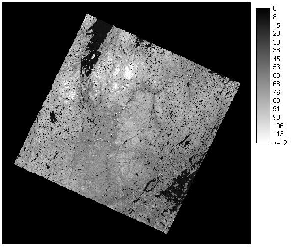
In order to perform training data collection, it is necessary to make false
colour composite images. The data characteristics for each of the seven
bands of the Landsat TM imagery is shown as an example below.
|
TM band
|
wavelength
|
characteristics
|
|
1
|
blue
|
Designed for water body penetration, making
it useful for coastal water mapping. Also useful for soil/vegetation discrimination,
forest type mapping. |
|
2
|
green
|
Designed to measure green reflectance peak of
vegetation for vegetation discrimination and vigor assessment |
|
3
|
Red
|
Designed to sense in a chlorophyll absorption
region aiding in plant species differentiation |
|
4
|
Near-IR
|
Useful for determining vegetation types, vigor,
biomass content, for delineating water bodies, and for soil moisture discrimination |
|
5
|
Mid-IR
|
Indicates moisture content of soil and vegetation.
Penetrates thin clouds. Good contrast between vegetation types. |
|
6
|
Thermal IR
|
Useful in vegetation stress analysis, soil moisture
discrimination, and thermal mapping applications |
|
7
|
Mid-IR
|
Useful for discrimination of mineral and rock
types. Also sensitive to vegetation moisture content. |
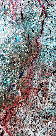
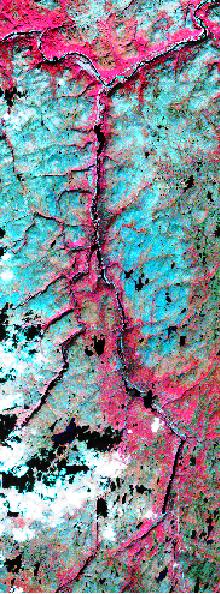
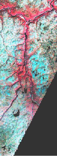
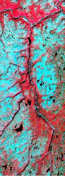
In this contract, a lot of band combinations are tested. We found TM
bands 4, 3, and 2 is a suitable combination for collecting training data.
It means that TM bands 4, 3, and 2 are combined to make false-color composite
images where band 4 represents red, band 3, green, and band 2, blue. This
band combination makes birch forest appear as shades of red. Heights will
be lighter blue. Water bodies will appear blue. Deep, clear water will
be dark blue to black in color, while sediment-laden or shallow waters
will appear lighter in color. Urban areas will appear blue-gray in color.
Clouds will be bright white. Figures 1a 1g show TM bands 4, 3, and 2
composite images of three dates (except for Vuotso) for two sites with
histogram equalization respectively.
The maximum likelihood classification (MLC) method was used in this study.
The maximum likelihood classification is based on the probability density
function associated with a particular training sample statistics. Pixels
are assigned to the most likely class based on a comparison of the posterior
probability that it belongs to each of the training sites statistics.
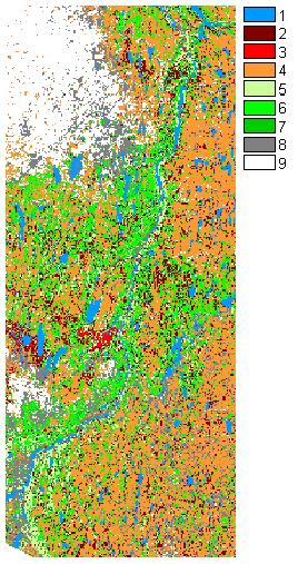
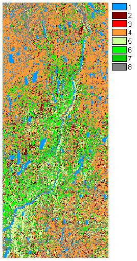
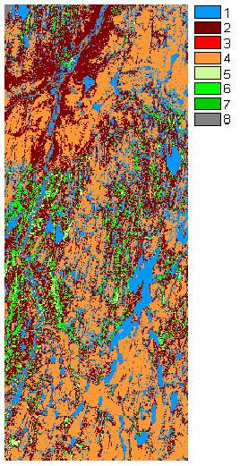
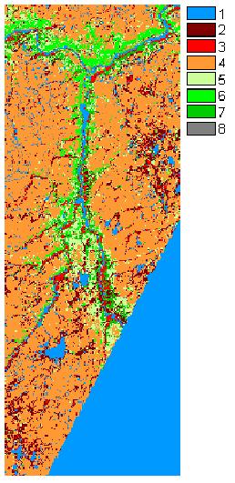
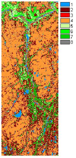
A two-level classification scheme was used in this contract work. The MLC
classification was carried out based on the 26 land-use types at the second
level of the scheme. Information about the first level was derived by aggregating
corresponding types at the second level. Among these land-use types, birch
forest types are the most important subjects. The land-use types at first
level are listed as following:
|
1
|
Water
|
|
2
|
bogs/wetlands |
|
3
|
mixed forests (incl. Pine) |
|
4
|
Heaths |
|
5
|
birch forest: richer type |
|
6
|
birch forest: cranberry-/crowberry-type (with
lichencover) |
|
7
|
birch forest: blueberry type |
|
8
|
Cultivated areas |
Traditional supervised training involves the selection of contiguous
pixels or blocks of pixel from representative locations across the image
as training samples. Selection of the training samples was aided by use
of 1:250,000 Maze vegetation map. The eight sets of training statistics
were used with the Maximum Likelihood Classifier (MLC). It must be noted
that same training sample pixels are used in three date images for each
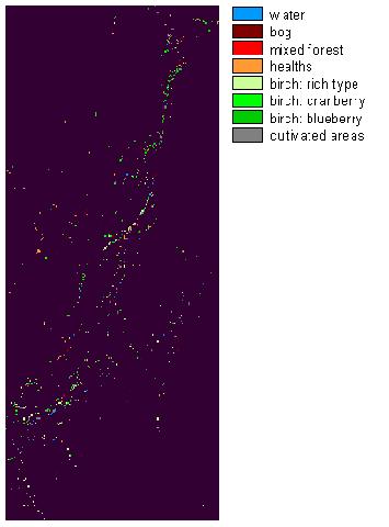
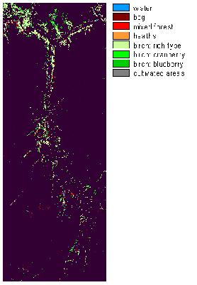
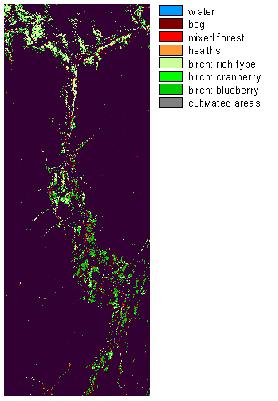
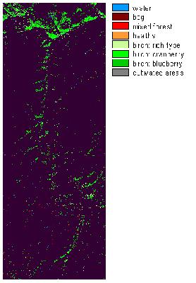
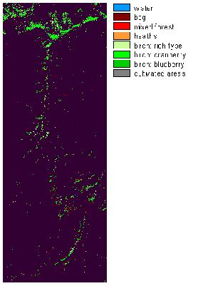
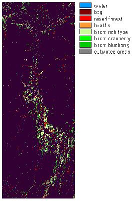
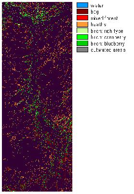
site. Figure 2a 2f show the first-level classified maps of three dates
for two sites (class labels refer to above descriptions).
-
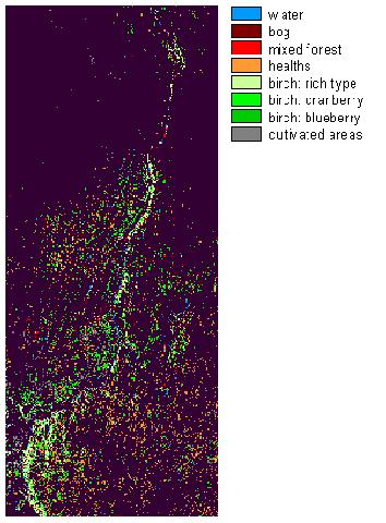
Post-classification change detection
Post-classification comparison change detection was selected to perform
land cover change detection in this contract work. Post-classification
comparison change detection is the most commonly used quantitative method
of change detection. It requires rectification and classification of each
remotely sensed image. These two maps are then compared on a pixel-by-pixel
basis using a change detection matrix. The advantage of this method includes
the detailed fromto information that can be extracted and the fact that
the classification map for the next base year is already complete (Jensen
1996). However, every error in the individual date classification map will
also be presented in the final change detection map (Rutchey and Velcheck
1994). Therefore, it is imperative that the individual classification maps
used in the post-classification change detection method be as accurate
as possible (Augenstein et al. 1991 ). As we know, the different
birch forest types are the most important subjects. This work shows some
results of change of the different birch forest types between different
dates in two sites: Masi and Vtsjokia (since Vuotso only has one date (1986)
TM imagery now, this sites image classification and change detection will
be done after the new dataset for other years come). Figures 3, 4, and
5 show the changes of three birch forest types and other land-use types
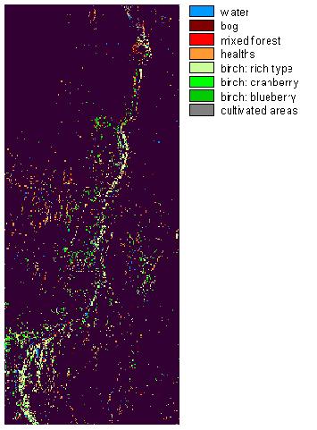
between 1987 and 1995 in Masi resepectively. Utsjokias changes between
1987 and 1995 are shown in figures 6, 7, and 8.
 |
 |
| Figure 3a. other land-use types to birch forest: rich types (1987 -
1995) in Masi |
Figure 3b. birch forest: rich types to other land-use types (1987 -
1995) in Masi |
 |
 |
| Figure 4a. other land-use types to birch forest: cranberry (1987 -
1995) in Masi |
Figure 4b. birch forest: cranberry to pther land-use types (1987 -
1995) in Masi |
 |
 |
| Figure 5a. other types to birch forest: blueberry (1987 ? 1995) in
Masi |
Figure 5b. birch forest: blueberry to other land-use (1987 ? 1995)
in Masi |
 |
 |
| Figure 6a. other land-use types to birch forest: rich types (1987 ?
2000) in Utsjokia |
Figure 6b. birch forest: rich types to other land-use types (1987 ?
2000) in Utsjokia |
 |
 |
| Figure 7a. other types to birch forest: cranberry (1987 ? 2000) in
Utsjokia |
Figure 7b. birch forest: cranberry to other types (1987 ? 2000) in
Utsjokia |
 |
 |
| Figure 8a. other types to birch forest: blueberry (1987 ? 2000) in
Utsjokia |
Figure 7b. birch forest: rich types to other types (1987 ? 2000) in
Utsjokia |